Binder Demo
Try out the package without installation (after loading, try clicking on README.Rmd in the Files tab).
Overview
The rEDM package is a collection of methods for Empirical Dynamic Modeling (EDM). EDM is based on the mathematical theory of recontructing attractor manifolds from time series data, with applications to forecasting, causal inference, and more. It is based on research software previously developed for the Sugihara Lab (University of California San Diego, Scripps Institution of Oceanography).
Installation
You can install rEDM from CRAN with:
OR from github with:
If you are on Windows, you may need to install Rtools first, so that you have access to a C++ compiler.
Example
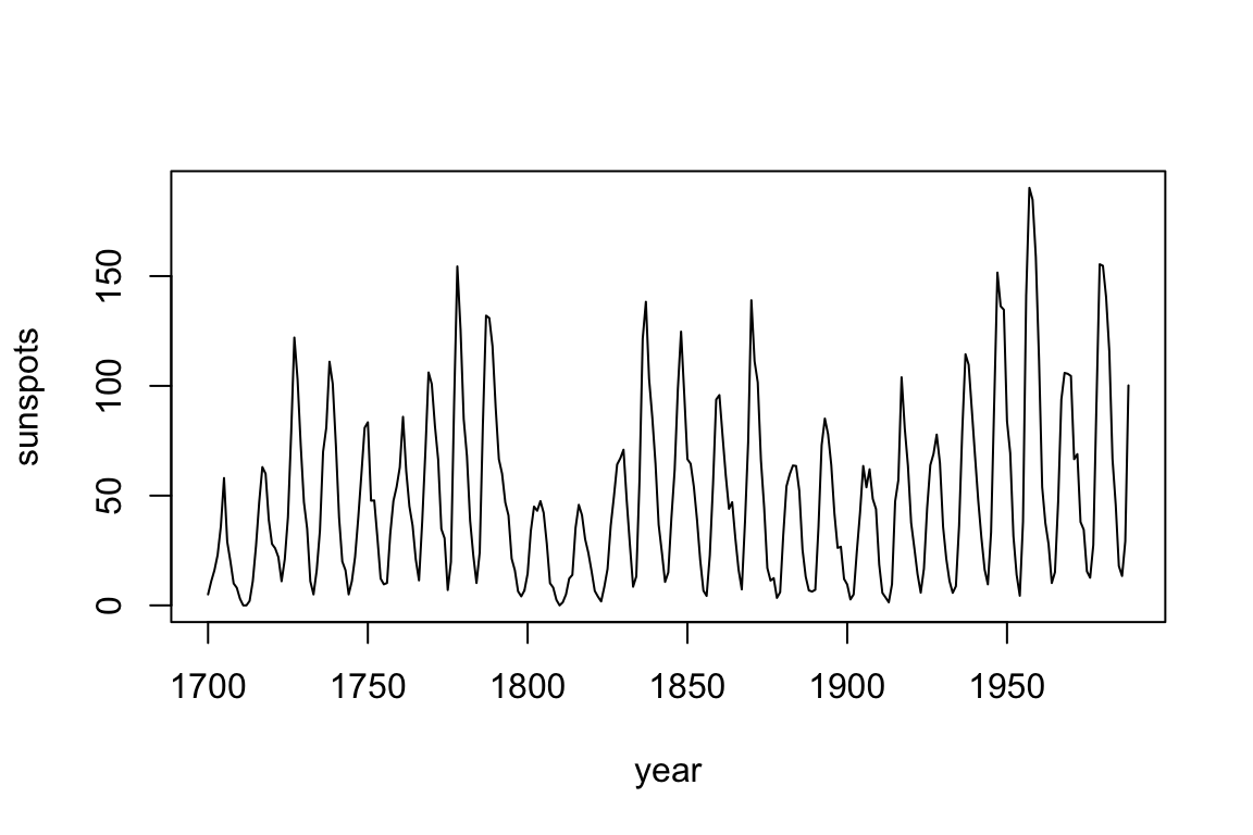
We begin by looking at annual time series of sunspots:
dat <- data.frame(yr = as.numeric(time(sunspot.year)),
                  sunspot_count = as.numeric(sunspot.year))

plot(dat$yr, dat$sunspot_count, type = "l",
     xlab = "year", ylab = "sunspots")
First, we use simplex to determine the optimal embedding dimension, E:
library(rEDM)                             # load the package

n <- NROW(dat)
lib <- c(1, floor(2/3 * n))               # indices for the first 2/3 of the time series
pred <- c(floor(2/3 * n) + 1, n)          # indices for the final 1/3 of the time series

output <- simplex(dat,                    # input data (for data.frames, uses 2nd column)
                  lib = lib, pred = lib,  # which portions of the data to train and predict
                  E = 1:10)               # embedding dimensions to try

summary(output[, 1:9])
#>        E              tau          tp          nn           num_pred
#>  Min.   : 1.00   Min.   :1   Min.   :1   Min.   : 2.00   Min.   :182.0
#>  1st Qu.: 3.25   1st Qu.:1   1st Qu.:1   1st Qu.: 4.25   1st Qu.:184.2
#>  Median : 5.50   Median :1   Median :1   Median : 6.50   Median :186.5
#>  Mean   : 5.50   Mean   :1   Mean   :1   Mean   : 6.50   Mean   :186.5
#>  3rd Qu.: 7.75   3rd Qu.:1   3rd Qu.:1   3rd Qu.: 8.75   3rd Qu.:188.8
#>  Max.   :10.00   Max.   :1   Max.   :1   Max.   :11.00   Max.   :191.0
#>       rho              mae             rmse            perc
#>  Min.   :0.7082   Min.   :10.17   Min.   :13.94   Min.   :1
#>  1st Qu.:0.8759   1st Qu.:10.78   1st Qu.:14.21   1st Qu.:1
#>  Median :0.9079   Median :11.32   Median :14.86   Median :1
#>  Mean   :0.8815   Mean   :12.15   Mean   :16.48   Mean   :1
#>  3rd Qu.:0.9172   3rd Qu.:12.72   3rd Qu.:17.42   3rd Qu.:1
#>  Max.   :0.9195   Max.   :18.23   Max.   :25.92   Max.   :1
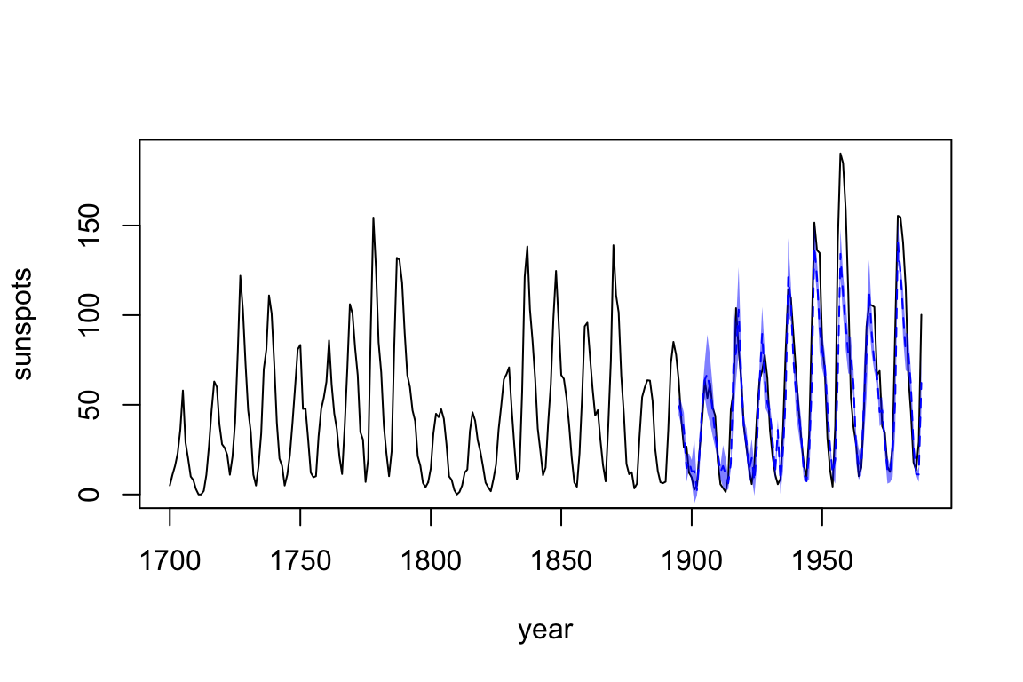
It looks like E = 3 or 4 is optimal. Since we generally want a simpler model, if possible, let’s go with E = 3 to forecast the remaining 1/3 of the data.
output <- simplex(dat,
                  lib = lib, pred = pred, # predict on last 1/3
                  E = 3,
                  stats_only = FALSE)     # return predictions, too

predictions <- na.omit(output$model_output[[1]])

plot(dat$yr, dat$sunspot_count, type = "l",
          xlab = "year", ylab = "sunspots")
lines(predictions$time, predictions$pred, col = "blue", lty = 2)
polygon(c(predictions$time, rev(predictions$time)),
        c(predictions$pred - sqrt(predictions$pred_var),
        rev(predictions$pred + sqrt(predictions$pred_var))),
        col = rgb(0, 0, 1, 0.5), border = NA)